Visualization and Interaction

Interactive Control Panel

A model can be manipulated and visualized in Jupyter Notebook by calling model.controlpanel(). By default this creates a slider for every constant in the model and gives them automatic ranges, but variables and/or ranges can be changed in the Settings tab or specified in the first argument to controlpanel().

Besides the default behaviour shown above, the control panel can also display custom analyses and plots via the fn_of_sol argument, which accepts a function (or list of functions) that take the solution as their input.

Plotting a 1D Sweep

Methods exist to facilitate creating, solving, and plotting the results of a single-variable sweep (see Sweeps for details). Example usage is as follows:

"Demonstrates manual and auto sweeping and plotting"
import matplotlib as mpl
mpl.use('Agg')
# comment out the imports above and `show()` to show figures in a window
import numpy as np
from gpkit import Model, Variable, units

x = Variable("x", "m", "Swept Variable")
y = Variable("y", "m^2", "Cost")
m = Model(y, [y >= (x/2)**-0.5 * units.m**2.5 + 1*units.m**2, y >= (x/2)**2])

# arguments are: model, swept: values, posnomial for y-axis
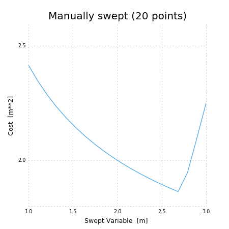
sol = m.sweep({x: np.linspace(1, 3, 20)}, verbosity=0)
f, ax = sol.plot(y)
ax.set_title("Manually swept (20 points)")
# f.show()
f.savefig("plot_sweep1d.png")

# arguments are: model, swept: (min, max, optional logtol), posnomial for y-axis
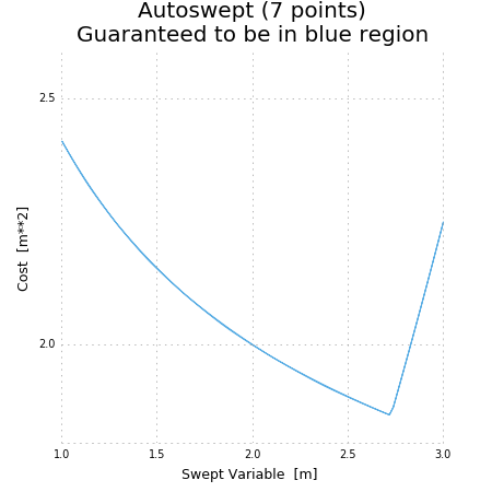
sol = m.autosweep({x: (1, 3)}, tol=0.001, verbosity=0)
f, ax = sol.plot(y)
ax.set_title("Autoswept (7 points)\nGuaranteed to be in blue region")
# f.show()
f.savefig("plot_autosweep1d.png")

Which results in: