BOX

Maximize volume while limiting the aspect ratios and area of the sides.

This is a simple demonstration of gpkit, based on an example from A Tutorial on Geometric Programming by Boyd et al..

Set up the modelling environment

First we’ll to import GPkit and turn on \(\LaTeX\) printing for GPkit variables and equations.

import gpkit
import gpkit.interactive
gpkit.interactive.init_printing()

Now we declare the optimisation parameters:

alpha = gpkit.Variable("\\alpha", 2, "-", "lower limit, wall aspect ratio")
beta = gpkit.Variable("\\beta", 10, "-", "upper limit, wall aspect ratio")
gamma = gpkit.Variable("\\gamma", 2, "-", "lower limit, floor aspect ratio")
delta = gpkit.Variable("\\delta", 10, "-", "upper limit, floor aspect ratio")
A_wall = gpkit.Variable("A_{wall}", 200, "m^2", "upper limit, wall area")
A_floor = gpkit.Variable("A_{floor}", 50, "m^2", "upper limit, floor area")

Next, we declare the decision variables:

var = gpkit.Variable # a convenient shorthand

h = var("h", "m", "height")
w = var("w", "m", "width")
d = var("d", "m", "depth")

Then we form equations of the system:

V = h*w*d
constraints = [A_wall >= 2*h*w + 2*h*d,
               A_floor >= w*d,
               h/w >= alpha,
               h/w <= beta,
               d/w >= gamma,
               d/w <= delta]

Formulate the optimisation problem

Here we write the optimisation problem as a standard form geometric program. Note that by putting \(\tfrac{1}{V}\) as our cost function, we are maximizing \(V\).

gp = gpkit.GP(1/V, constraints)

Now we can check that our equations are correct by using the built-in latex printing.

gp

\[\begin{split}\begin{array}[ll] \text{} \text{minimize} & \frac{1}{d h w}\mathrm{\left[ \tfrac{1}{m^{3}} \right]} \\ \text{subject to} & A_{wall} \geq 2d h + 2h w \\ & A_{floor} \geq d w \\ & \alpha \leq \frac{h}{w} \\ & \beta \geq \frac{h}{w} \\ & \gamma \leq \frac{d}{w} \\ & \delta \geq \frac{d}{w} \\ \text{substituting} & A_{floor} = 50 \\ & A_{wall} = 200 \\ & \alpha = 2 \\ & \beta = 10 \\ & \delta = 10 \\ & \gamma = 2 \\ \end{array}\end{split}\]

That looks fine, but let’s change \(A_{floor}\) to \(100\), just for fun.

Note that replace=True will be needed, since \(A_{floor}\) has already been substituted in.

gp.sub(A_floor, 100, replace=True) # (var, val) substitution syntax

And heck, why not change \(\alpha\) and \(\gamma\) to \(1\) while we’re at it?

gp.sub({alpha: 1, gamma: 1}, replace=True) # ({var1: val1, var2: val2}) substitution syntax

Now check that those changes took:

gp

\[\begin{split}\begin{array}[ll] \text{} \text{minimize} & \frac{1}{d h w}\mathrm{\left[ \tfrac{1}{m^{3}} \right]} \\ \text{subject to} & A_{wall} \geq 2d h + 2h w \\ & A_{floor} \geq d w \\ & \alpha \leq \frac{h}{w} \\ & \beta \geq \frac{h}{w} \\ & \gamma \leq \frac{d}{w} \\ & \delta \geq \frac{d}{w} \\ \text{substituting} & A_{floor} = 100 \\ & A_{wall} = 200 \\ & \alpha = 1 \\ & \beta = 10 \\ & \delta = 10 \\ & \gamma = 1 \\ \end{array}\end{split}\]

Looks good!

Solve the GP

sol = gp.solve()

Using solver 'cvxopt'
Solving took 0.0184 seconds

Analyse results

print sol.table()

0.0025981 : Cost
          | Free variables
        d : 11.5     [m] depth
        h : 5.77     [m] height
        w : 5.77     [m] width
          |
          | Constants
A_{floor} : 100      [m**2] upper limit, floor area
 A_{wall} : 200      [m**2] upper limit, wall area
   alpha : 1        [-] lower limit, wall aspect ratio
    beta : 10       [-] upper limit, wall aspect ratio
   delta : 10       [-] upper limit, floor aspect ratio
   gamma : 1        [-] lower limit, floor aspect ratio
          |
          | Constant sensitivities
 A_{wall} : -1.5     [-] upper limit, wall area
   alpha : 0.5      [-] lower limit, wall aspect ratio
          |

Hmm, why didn’t \(A_{floor}\) show up in the sensitivities list?

sol.senssubinto(A_floor)

-3.4698494246624108e-09

Its sensitivity is tiny; changing it near this value doesn’t affect the cost at all; that constraint is loose! Let’s sweep over a range of \(A_{floor}\) values to figure out where it becomes loose.

Sweep and plot results

Import the plotting library matplotlib and the math library numpy:

%matplotlib inline
%config InlineBackend.figure_format = 'retina' # for high-DPI displays
import matplotlib.pyplot as plt
import numpy as np

Solve for values of \(A_{floor}\) from 10 to 100 using a “sweep” substitution:

gp.sub(A_floor, ('sweep', np.linspace(10, 100, 50)), replace=True)
sol = gp.solve()
print sol.table()

Using solver 'cvxopt'
Sweeping 1 variables over 50 passes
Solving took 0.547 seconds
 0.0032211 : Cost (average of 50 values)
           | Free variables (average)
         d : 8.33     [m] depth
         h : 7.74     [m] height
         w : 5.69     [m] width
           |
           | Constants (average)
 A_{floor} : 55       [m**2] upper limit, floor area
  A_{wall} : 200      [m**2] upper limit, wall area
    alpha : 1        [-] lower limit, wall aspect ratio
     beta : 10       [-] upper limit, wall aspect ratio
    delta : 10       [-] upper limit, floor aspect ratio
    gamma : 1        [-] lower limit, floor aspect ratio
           |
           | Constant sensitivities (average)
 A_{floor} : -0.274   [-] upper limit, floor area
  A_{wall} : -1.23    [-] upper limit, wall area
    alpha : 0.226    [-] lower limit, wall aspect ratio
           |

It seems we got some sensitivity out of \(A_{floor}\) on average over these points; let’s plot it:

plt.plot(sol(A_floor), sol(d), linewidth=1, alpha=0.5)
plt.plot(sol(A_floor), sol(h), linewidth=1, alpha=0.5)
plt.plot(sol(A_floor), sol(w), '--', linewidth=2, alpha=0.5)
plt.legend(['depth', 'height', 'width'])
plt.ylabel("Optimal dimensions [m]")
_ = plt.xlabel("A_floor [m^2]") # the _ catches the returned label object, since we don't need it

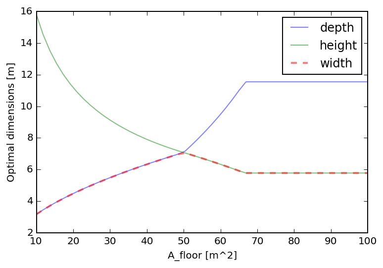
There’s an interesting elbow when \(A_{floor} \approx 50 \mathrm{\ m^2}\).

Interactive analysis

Let’s investigate it with the cadtoons library. Running cadtoon.py box.svg in this folder creates an interactive SVG graphic for us.

First, import the functions to display HTML in iPython Notebook, and the ractivejs library.

from IPython.display import HTML, display
from string import Template

Then write controls that link the optimization to the animation. It’s generally very helpful to play around with with writing constraints in the cadtoons sandbox before copying the javascript code from there to iPython.

ractor = Template("""
var w = $w/10,
    h = $h/10,
    d = $d/10""")

def ractorfn(sol):
    return ractor.substitute(w=sol(w), d=sol(d), h=sol(h))

constraints="""
var dw = 50*(w-1),
    dh = 50*(h-1),
    dd = 50*(d-1)

r.plan.scalex = w
r.plan.scaley = d

r.top.scalex = w
r.top.scaley = h
r.top.y = -dh -dd
r.bottom.scalex = w
r.bottom.scaley = h
r.bottom.y = dh + dd

r.left.scalex = h
r.left.scaley = d
r.left.x = -dh - dw
r.right.scalex = h
r.right.scaley = d
r.right.x = dh + dw """

def ractivefn(gp):
    sol = gp.solution
    live = "<script>" + ractorfn(sol) + constraints + "</script>"
    display(HTML(live))
    # if you enable the line below, you can try navigating the sliders by sensitivities
    # print sol.table(["cost", "sensitivities"])

Now that the display window has been created, let’s use an iPython widget to explore the “design space” of our box. This widget runs the gpkit solver every time a slider is changed, so you only solve the points you see.

with open("box.gpkit", 'r') as file:
    display(HTML(file.read()))
display(HTML(display(HTML("<style> #ractivecontainer"
             "{position:absolute; height: 0;"
             "right: 0; top: 5em;} </style>"))))

<IPython.core.display.HTML at 0x7fd2dce97850>

gpkit.interactive.widget(gp, ractivefn, {
    "A_{floor}": (10, 1000, 10), "A_{wall}": (10, 1000, 10),
    "\\delta": (0.1, 20, 0.1), "\\gamma": (0.1, 20, 0.1),
    "\\alpha": (0.1, 20, 0.1), "\\beta": (0.1, 20, 0.1), })

Now that we’ve found a good range to explore, we’ll make and interactive javascript widget that presolves all options and works in a iPython notebook hosted by nbviewer.

gpkit.interactive.jswidget(gp, ractorfn, constraints, {
    "A_{floor}": (10, 100, 10), "A_{wall}": (10, 210, 20),
    "\\delta": (1, 10, 3), "\\gamma": (1, 10, 3),
    "\\alpha": (1, 10, 3), "\\beta": (1, 10, 3), })

This concludes the Box example. Try playing around with the sliders up above until you’re bored of this simple system; then check out one of the other examples. Thanks for reading!

Import CSS for nbviewer

If you have a local iPython stylesheet installed, this will add it to the iPython Notebook:

from IPython import utils
from IPython.core.display import HTML
import os
def css_styling():
    """Load default custom.css file from ipython profile"""
    base = utils.path.get_ipython_dir()
    styles = ("<style>\n%s\n</style>" %
              open(os.path.join(base,'profile_default/static/custom/custom.css'),'r').read())
    return HTML(styles)
css_styling()