
AIRPLANE FUEL
Minimize fuel needed for a plane that can sprint and land quickly.
Set up the modelling environment
First we’ll to import GPkit and turn on \(\LaTeX\) printing for GPkit variables and equations.
import numpy as np
import gpkit
import gpkit.interactive
gpkit.interactive.init_printing()
declare constants
mon = gpkit.Variable
vec = gpkit.VectorVariable

N_lift         = mon("N_{lift}", 6.0, "-", "Wing loading multiplier")
pi             = mon("\\pi", np.pi, "-", "Half of the circle constant")
sigma_max      = mon("\\sigma_{max}", 250e6, "Pa", "Allowable stress, 6061-T6")
sigma_maxshear = mon("\\sigma_{max,shear}", 167e6, "Pa", "Allowable shear stress")
g              = mon("g", 9.8, "m/s^2", "Gravitational constant")
w              = mon("w", 0.5, "-", "Wing-box width/chord")
r_h            = mon("r_h", 0.75, "-", "Wing strut taper parameter")
f_wadd         = mon("f_{wadd}", 2, "-", "Wing added weight fraction")
W_fixed        = mon("W_{fixed}", 14.7e3, "N", "Fixed weight")
C_Lmax         = mon("C_{L,max}", 1.5, "-", "Maximum C_L, flaps down")
rho            = mon("\\rho", 0.91, "kg/m^3", "Air density, 3000m")
rho_sl         = mon("\\rho_{sl}", 1.23, "kg/m^3", "Air density, sea level")
rho_alum       = mon("\\rho_{alum}", 2700, "kg/m^3", "Density of aluminum")
mu             = mon("\\mu", 1.69e-5, "kg/m/s", "Dynamic viscosity, 3000m")
e              = mon("e", 0.95, "-", "Wing spanwise efficiency")
A_prop         = mon("A_{prop}", 0.785, "m^2", "Propeller disk area")
eta_eng        = mon("\\eta_{eng}", 0.35, "-", "Engine efficiency")
eta_v          = mon("\\eta_v", 0.85, "-", "Propeller viscous efficiency")
h_fuel         = mon("h_{fuel}", 42e6, "J/kg", "fuel heating value")
V_sprint_reqt  = mon("V_{sprintreqt}", 150, "m/s", "sprint speed requirement")
W_pay          = mon("W_{pay}", 500*9.81, "N")
R_min          = mon("R_{min}", 1e6, "m", "Minimum airplane range")
V_stallmax     = mon("V_{stall,max}", 40, "m/s", "Stall speed")
# sweep variables
R_min          = mon("R_{min}", np.linspace(1e6, 1e7, 10), "m", "Minimum airplane range")
V_stallmax     = mon("V_{stall,max}", np.linspace(30, 50, 10), "m/s", "Stall speed")
declare free variables
V        = vec(3, "V", "m/s", "Flight speed")
C_L      = vec(3, "C_L", "-", "Wing lift coefficent")
C_D      = vec(3, "C_D", "-", "Wing drag coefficent")
C_Dfuse  = vec(3, "C_{D_{fuse}}", "-", "Fuselage drag coefficent")
C_Dp     = vec(3, "C_{D_p}", "-", "drag model parameter")
C_Di     = vec(3, "C_{D_i}", "-", "drag model parameter")
T        = vec(3, "T", "N", "Thrust force")
Re       = vec(3, "Re", "-", "Reynold's number")
W        = vec(3, "W", "N", "Aircraft weight")
eta_i    = vec(3, "\\eta_i", "-", "Aircraft efficiency")
eta_prop = vec(3, "\\eta_{prop}", "-")
eta_0    = vec(3, "\\eta_0", "-")
W_fuel   = vec(2, "W_{fuel}", "N", "Fuel weight")
z_bre    = vec(2, "z_{bre}", "-")
S        = mon("S", "m^2", "Wing area")
R        = mon("R", "m", "Airplane range")
A        = mon("A", "-", "Aspect Ratio")
I_cap    = mon("I_{cap}", "m^4", "Spar cap area moment of inertia per unit chord")
M_rbar   = mon("\\bar{M}_r", "-")
P_max    = mon("P_{max}", "W")
V_stall  = mon("V_{stall}", "m/s")
nu       = mon("\\nu", "-")
p        = mon("p", "-")
q        = mon("q", "-")
tau      = mon("\\tau", "-")
t_cap    = mon("t_{cap}", "-")
t_web    = mon("t_{web}", "-")
W_cap    = mon("W_{cap}", "N")
W_zfw    = mon("W_{zfw}", "N", "Zero fuel weight")
W_eng    = mon("W_{eng}", "N")
W_mto    = mon("W_{mto}", "N", "Maximum takeoff weight")
W_pay    = mon("W_{pay}", "N")
W_tw     = mon("W_{tw}", "N")
W_web    = mon("W_{web}", "N")
W_wing   = mon("W_{wing}", "N")
Let’s check that the vector constraints are working:
W == 0.5*rho*C_L*S*V**2
Looks good!
Form the optimization problem
In the 3-element vector variables, indexs 0, 1, and 2 are the outbound, return and sprint flights.
steady_level_flight = (W == 0.5*rho*C_L*S*V**2,
                       T >= 0.5*rho*C_D*S*V**2,
                       Re == (rho/mu)*V*(S/A)**0.5)

landing_fc = (W_mto <= 0.5*rho_sl*V_stall**2*C_Lmax*S,
              V_stall <= V_stallmax)

sprint_fc = (P_max >= T[2]*V[2]/eta_0[2],
             V[2] >= V_sprint_reqt)

drag_model = (C_D >= (0.05/S)*gpkit.units.m**2 +C_Dp + C_L**2/(pi*e*A),
              1 >= (2.56*C_L**5.88/(Re**1.54*tau**3.32*C_Dp**2.62) +
                   3.8e-9*tau**6.23/(C_L**0.92*Re**1.38*C_Dp**9.57) +
                   2.2e-3*Re**0.14*tau**0.033/(C_L**0.01*C_Dp**0.73) +
                   1.19e4*C_L**9.78*tau**1.76/(Re*C_Dp**0.91) +
                   6.14e-6*C_L**6.53/(Re**0.99*tau**0.52*C_Dp**5.19)))

propulsive_efficiency = (eta_0 <= eta_eng*eta_prop,
                         eta_prop <= eta_i*eta_v,
                         4*eta_i + T*eta_i**2/(0.5*rho*V**2*A_prop) <= 4)

# 4th order taylor approximation for e^x
z_bre_sum = 0
for i in range(1,5):
    z_bre_sum += z_bre**i/np.math.factorial(i)

range_constraints = (R >= R_min,
                     z_bre >= g*R*T[:2]/(h_fuel*eta_0[:2]*W[:2]),
                     W_fuel/W[:2] >= z_bre_sum)

weight_relations = (W_pay >= 500*g*gpkit.units.kg,
                    W_tw >= W_fixed + W_pay + W_eng,
                    W_zfw >= W_tw + W_wing,
                    W_eng >= 0.0372*P_max**0.8083 * gpkit.units.parse_expression('N/W^0.8083'),
                    W_wing/f_wadd >= W_cap + W_web,
                    W[0] >= W_zfw + W_fuel[1],
                    W[1] >= W_zfw,
                    W_mto >= W[0] + W_fuel[0],
                    W[2] == W[0])

wing_structural_model = (2*q >= 1 + p,
                         p >= 1.9,
                         tau <= 0.15,
                         M_rbar >= W_tw*A*p/(24*gpkit.units.N),
                         .92**2/2.*w*tau**2*t_cap >= I_cap * gpkit.units.m**-4 + .92*w*tau*t_cap**2,
                         8 >= N_lift*M_rbar*A*q**2*tau/S/I_cap/sigma_max * gpkit.units.parse_expression('Pa*m**6'),
                         12 >= A*W_tw*N_lift*q**2/tau/S/t_web/sigma_maxshear,
                         nu**3.94 >= .86*p**-2.38 + .14*p**0.56,
                         W_cap >= 8*rho_alum*g*w*t_cap*S**1.5*nu/3/A**.5,
                         W_web >= 8*rho_alum*g*r_h*tau*t_web*S**1.5*nu/3/A**.5
                         )
eqns = (weight_relations + range_constraints + propulsive_efficiency
        + drag_model + steady_level_flight + landing_fc + sprint_fc + wing_structural_model)

gp = gpkit.GP(W_fuel.sum(), eqns)
Design a hundred airplanes
sol = gp.solve()
Using solver 'cvxopt'
Sweeping 2 variables over 100 passes
Solving took 9.96 seconds
The “local model” is the power-law tangent to the Pareto frontier, gleaned from sensitivities.
sol["local_model"][0].sub(gp.substitutions)
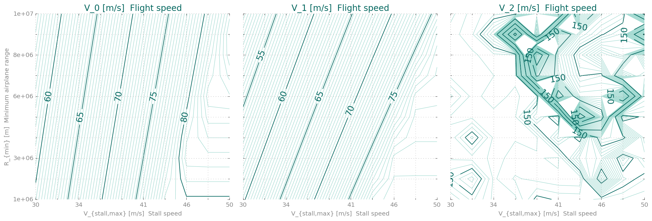
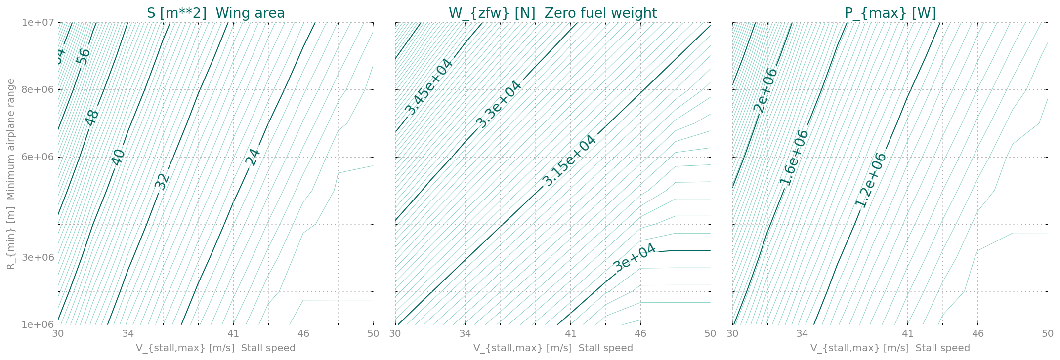
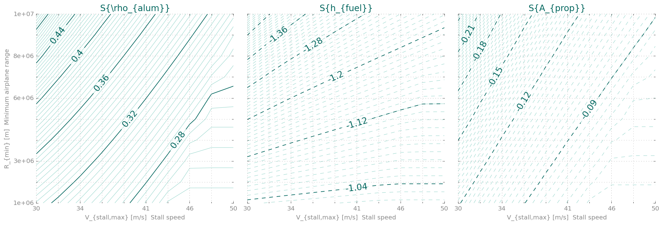
plot design frontiers
%matplotlib inline
%config InlineBackend.figure_format = 'retina'

plot_frontiers = gpkit.interactive.plot_frontiers
plot_frontiers(gp, [V[0], V[1], V[2]])
plot_frontiers(gp, [S, W_zfw, P_max])
plot_frontiers(gp, ['S{\\rho_{alum}}', 'S{h_{fuel}}', 'S{A_{prop}}'])
Interactive analysis
Let’s investigate it with the cadtoons library. Running cadtoon.py flightconditions.svg in this folder creates an interactive SVG graphic for us.
First, import the functions to display HTML in iPython Notebook, and the ractivejs library.
from IPython.display import HTML, display
from string import Template
ractor = Template("""
var W_eng = $W_eng,
    lam = $lam

r.shearinner.scalex = 1-$tcap*10
r.shearinner.scaley = 1-$tweb*100
r.airfoil.scaley = $tau/0.13
r.fuse.scalex = $W_fus/24000
r.wing.scalex = $b/2/14
r.wing.scaley = $cr*1.21
""")

def ractorfn(sol):
    return ractor.substitute(lam = 0.5*(sol(p) - 1),
                             b = sol((S*A)**0.5),
                             cr = sol(2/(1+0.5*(sol(p) - 1))*(S/A)**0.5),
                             tcap = sol(t_cap/tau),
                             tweb = sol(t_web/w),
                             tau = sol(tau),
                             W_eng = sol(W_eng),
                             W_fus = sol(W_mto) - sol(W_wing) - sol(W_eng))

constraints = """
r.engine1.scale = Math.pow(W_eng/3000, 2/3)
r.engine2.scale = Math.pow(W_eng/3000, 2/3)
r.engine1.y = 6*lam
r.engine2.y = 6*lam
r.wingrect.scaley = 1-lam
r.wingrect.y = -6 + 5*lam
r.wingtaper.scaley = lam
r.wingtaper.y = 5*lam
"""

def ractivefn(gp):
    sol = gp.solution
    live = "<script>" + ractorfn(sol) + constraints + "</script>"
    display(HTML(live))
    # if you enable the line below, you can try navigating the sliders by sensitivities
    # print sol.table(["cost", "sensitivities"])
with open("flightconditions.gpkit", 'r') as file:
    display(HTML(file.read()))
display(HTML("<style> #ractivecontainer"
             "{position:absolute; height: 0;"
             "right: 0; top: -6em;} </style>"))
gpkit.interactive.widget(gp, ractivefn,
         {"V_{stall,max}": (20, 50, 1),
          "R_{min}": (1e6, 1e7, 0.5e6)})
gpkit.interactive.jswidget(gp, ractorfn,
                           constraints,
           {"V_{stall,max}": (20, 50, 3),
            "R_{min}": (1e6, 1e7, 1e6)})
This concludes the Box example. Try playing around with the sliders up above until you’re bored of this system; then check out one of the other examples. Thanks for reading!
Import CSS for nbviewer
If you have a local iPython stylesheet installed, this will add it to the iPython Notebook:
from IPython import utils
from IPython.core.display import HTML
import os
def css_styling():
    """Load default custom.css file from ipython profile"""
    base = utils.path.get_ipython_dir()
    styles = "<style>\n%s\n</style>" % (open(os.path.join(base,'profile_default/static/custom/custom.css'),'r').read())
    return HTML(styles)
css_styling()