Visualization and Interaction
Code in this section uses the CE solar model except where noted otherwise.
Model and Variable Breakdowns
Model breakdowns (similar to the sankey diagrams below) show the hierarchy of a model scaled by the sensitivity of its constraints and fixed variables.
Variable breakdowns show how a variable “breaks down” into smaller expressions.
For example if the constraint x_total >= x1 + x2 is tight (that is, has a sensitivity greater than zero, indicating that the right hand side is “pushing” against the left), then x_total can be said to “break down” into x1 and x2, each of which may have their own breakdowns. If multiple constraints break down a variable, the most sensitive one is chosen; if none do, than constraints such as 1 >= x1/x_total + x2/x_total will be rearranged in an attempt to create a valid breakdown constraint like that above.
"An example to show off Breakdowns"
import os
import sys
import pickle
import pint
from packaging import version
from gpkit.breakdowns import Breakdowns

dirpath = os.path.dirname(os.path.realpath(__file__)) + os.sep
if version.parse(pint.__version__) >= version.parse("0.13"):
    sol = pickle.load(open(dirpath+"solar_13.p", "rb"))
elif version.parse(pint.__version__) >= version.parse("0.12"):
    sol = pickle.load(open(dirpath+"solar_12.p", "rb"))
elif version.parse(pint.__version__) >= version.parse("0.10"):
    sol = pickle.load(open(dirpath+"solar_10.p", "rb"))
elif version.parse(pint.__version__) == version.parse("0.9"):
    sol = pickle.load(open(dirpath+"solar.p", "rb"))
else:
    sol = None

# our Miniconda windows test platform can't print unicode
if sys.platform[:3] != "win" and sol is not None:
    # the code to create solar.p is in ./breakdowns/solartest.py
    bds = Breakdowns(sol)

    print("Cost breakdown (as seen in solution tables)")
    print("==============")
    bds.plot("cost")

    print("Variable breakdowns (note the two methods of access)")
    print("===================")
    varkey, = sol["variables"].keymap[("Mission.FlightSegment.AircraftPerf"
                                       ".AircraftDrag.Poper")]
    bds.plot(varkey)
    bds.plot("AircraftPerf.AircraftDrag.MotorPerf.Q")

    print("Combining the two above by increasing maxwidth")
    print("----------------------------------------------")
    bds.plot("AircraftPerf.AircraftDrag.Poper", maxwidth=105)

    print("Model sensitivity breakdowns (note the two methods of access)")
    print("============================")
    bds.plot("model sensitivities")
    bds.plot("Aircraft")

    print("Exhaustive variable breakdown traces (and configuration arguments)")
    print("====================================")
    # often useful as a reference point when reading traces
    bds.plot("AircraftPerf.AircraftDrag.Poper", height=12)
    # includes factors, can be useful for reading traces as well
    bds.plot("AircraftPerf.AircraftDrag.Poper", showlegend=True)
    print("\nPermissivity = 2 (the default)")
    print("----------------")
    bds.trace("AircraftPerf.AircraftDrag.Poper")
    print("\nPermissivity = 1 (stops at Pelec = v·i)")
    print("----------------")
    bds.trace("AircraftPerf.AircraftDrag.Poper", permissivity=1)

    # you can also produce Plotly treemaps/icicle plots of your breakdowns
    fig = bds.treemap("model sensitivities", returnfig=True)
    fig = bds.icicle("cost", returnfig=True)
    # uncommenting any of the below makes and shows the plot directly
    # bds.icicle("model sensitivities")
    # bds.treemap("cost")
Cost breakdown (as seen in solution tables)
==============
┃┓ ┓ ┓
┃┃ ┃ ┃
┃┃ ┃ ┃
┃┃ ┃ ┃
┃┃ ┃ ┃
┃┃ ┣╸Battery.W ┣╸Battery.E╶⎨
┃┃ ┃ (370lbf) ┃ (165,913kJ)
┃┃ ┃ ┃
┃┃ ┃ ┃
Cost╺┫┃ ┃ ┃
(699lbf) ┃┣╸Wtotal ┛ ┛
┃┃ (699lbf) ┓ ┓
┃┃ ┃ ┣╸Wing.BoxSpar.W╶⎨
┃┃ ┣╸Wing.W ┛ (96.1lbf)
┃┃ ┛ (139lbf) ┣╸Wing.WingSecondStruct.W╶⎨
┃┃ ┣╸Motor.W╶⎨
┃┃ ┣╸SolarCells.W╶⎨
┃┃ ┣╸Empennage.W
┃┃ ┣╸Wavn
┃┛ ┣╸[6 terms]
Variable breakdowns (note the two methods of access)
===================
┃┓ ┓ ┓
┃┃ ┃ ┃
┃┃ ┃ ┃
┃┃ ┃ ┃
┃┃ ┃ ┃
┃┃ ┃ ┃
┃┃ ┃ ┣╸MotorPerf.Q╶⎨
AircraftPerf.AircraftDrag.Poper╺┫┣╸MotorPerf.Pelec ┣╸MotorPerf.i ┃ (4.8N·m)
(3,194W) ┃┃ (0.685kW) ┃ (36.8A) ┃
┃┃ ┃ ┃
┃┃ ┃ ┃
┃┃ ┃ ┛
┃┃ ┃ ┣╸i0
┃┛ ┛ ┛ (4.5A, fixed)
┃┣╸Pavn
┃┣╸Ppay
┃┓
AircraftPerf.AircraftDrag.MotorPerf.Q╺┫┃
(4.8N·m) ┃┣╸..ActuatorProp.CP
┃┛ (0.00291)
Combining the two above by increasing maxwidth
----------------------------------------------
┃┓ ┓ ┓ ┓
┃┃ ┃ ┃ ┃
┃┃ ┃ ┃ ┃
┃┃ ┃ ┃ ┃
┃┃ ┃ ┃ ┃
┃┃ ┃ ┃ ┃
┃┃ ┃ ┣╸MotorPerf.Q ┣╸ActuatorProp.CP
AircraftPerf.AircraftDrag.Poper╺┫┣╸MotorPerf.Pelec ┣╸MotorPerf.i ┃ (4.8N·m) ┃ (0.00291)
(3,194W) ┃┃ (0.685kW) ┃ (36.8A) ┃ ┃
┃┃ ┃ ┃ ┃
┃┃ ┃ ┃ ┃
┃┃ ┃ ┛ ┛
┃┃ ┃ ┣╸i0
┃┛ ┛ ┛ (4.5A, fixed)
┃┣╸Pavn
┃┣╸Ppay
Model sensitivity breakdowns (note the two methods of access)
============================
┃┓ ┓ ┓ ┓ ┓
┃┃ ┃ ┃ ┃ ┃
┃┃ ┃ ┃ ┃ ┣╸ActuatorProp╶⎨
┃┃ ┃ ┃ ┃ ┛
┃┃ ┃ ┣╸AircraftPerf ┣╸AircraftDrag ┣╸MotorPerf╶⎨
┃┃ ┃ ┃ ┃ ┓
┃┣╸Mission ┣╸FlightSegment ┃ ┃ ┣╸[17 terms]
┃┃ ┃ ┛ ┛ ┛
┃┃ ┃ ┣╸FlightState╶⎨
Model╺┫┃ ┃ ┣╸GustL╶⎨
┃┃ ┃ ┣╸SteadyLevelFlight╶⎨
┃┃ ┛ ┣╸[49 terms]
┃┛ ┣╸Climb╶⎨
┃┓
┃┃
┃┃
┃┣╸Aircraft╶⎨
┃┃
┃┛
┃┣╸g = 9.81m/s²
┃┓ ┣╸etadischarge = 0.98
┃┃ ┛
┃┃ ┣╸W ≥ E·minSOC/hbatt/etaRTE/etapack·g
┃┃ ┣╸etaRTE = 0.95
┃┣╸Battery ┣╸etapack = 0.85
┃┃ ┣╸hbatt = 350W·hr/kg
┃┃ ┣╸minSOC = 1.03
┃┛ ┛
┃┓
Aircraft╺┫┃
┃┣╸Wing╶⎨
┃┃
┃┛
┃┣╸Wtotal/mfac ≥ Fuselage.W[0,0] + Fuselage.W[1,0] + Fuselage.W[2,0] …
┃┛
┃┣╸mfac = 1.05
┃┛
┃┣╸Empennage╶⎨
┃┣╸[23 terms]
┃┛
Exhaustive variable breakdown traces (and configuration arguments)
====================================
┃┓ ┓ ┓
┃┃ ┃ ┃
┃┃ ┃ ┃
┃┃ ┃ ┃
┃┃ ┃ ┃
AircraftPerf.AircraftDrag.Poper╺┫┣╸MotorPerf.Pelec ┣╸MotorPerf.i ┣╸MotorPerf.Q╶⎨
(3,194W) ┃┃ (0.685kW) ┃ (36.8A) ┃ (4.8N·m)
┃┃ ┃ ┃
┃┃ ┃ ┃
┃┃ ┃ ┛
┃┛ ┛ ┣╸i0
┃┣╸Pavn
┃╤╤┯╤┯╤┯┯╤┓
┃╎╎│╎│╎││╎┃
┃╎╎│╎│╎││╎┃
┃╎╎│╎│╎││╎┃
┃╎╎│╎│╎││╎┃
┃╎╎│╎│╎││╎┃
┃╎╎│╎│DCBA┣╸ActuatorProp.CP
AircraftPerf.AircraftDrag.Poper╺┫╎HGFE╎││╎┃ (0.00291)
(3,194W) ┃J╎│╎│╎││╎┃
┃╎╎│╎│╎││╎┃
┃╎╎│╎│╎││╎┃
┃╎╎│╎│╧┷┷╧┛
┃╎╎│╎│┣╸i0 (4.5A, fixed)
┃╎╧┷╧┷┛
┃╎┣╸Pavn (200W, fixed)
┃╧┣╸Ppay (100W, fixed)
A 4.53e-05·FlightState.rho·ActuatorProp.omega²·Propeller.R⁵ ×1,653N·m [free factor]
B ActuatorProp.Q = 4.8N·m
C MotorPerf.Q = 4.8N·m
D Kv ×64.2rpm/V [free factor]
E MotorPerf.i = 36.8A
F MotorPerf.v ×18.6V [free factor]
G MotorPerf.Pelec = 0.685kW
H Nprop ×4, fixed
J mpower ×1.05, fixed
Permissivity = 2 (the default)
----------------
AircraftPerf.AircraftDrag.Poper (3,194W)
which in: Poper/mpower ≥ Pavn + Ppay + Pelec·Nprop (sensitivity +5.6)
{ through a factor of AircraftPerf.AircraftDrag.mpower (1.05, fixed) }
breaks down into 3 monomials:
1) forming 90% of the RHS and 90% of the total:
{ through a factor of Nprop (4, fixed) }
AircraftPerf.AircraftDrag.MotorPerf.Pelec (0.685kW)
which in: Pelec = v·i (sensitivity -5.1)
breaks down into:
{ through a factor of AircraftPerf.AircraftDrag.MotorPerf.v (18.6V) }
AircraftPerf.AircraftDrag.MotorPerf.i (36.8A)
which in: i ≥ Q·Kv + i0 (sensitivity +5.4)
breaks down into 2 monomials:
1) forming 87% of the RHS and 79% of the total:
{ through a factor of Kv (64.2rpm/V) }
AircraftPerf.AircraftDrag.MotorPerf.Q (4.8N·m)
which in: Q = Q (sensitivity -4.7)
breaks down into:
AircraftPerf.AircraftDrag.ActuatorProp.Q (4.8N·m)
which in: CP ≤ Q·omega/(0.5·rho·(omega·R)³·π·R²) (sensitivity +4.7)
{ through a factor of 4.53e-05·FlightState.rho·AircraftPerf.AircraftDrag.ActuatorProp.omega²·Propeller.R⁵ (1,653N·m) }
breaks down into:
AircraftPerf.AircraftDrag.ActuatorProp.CP (0.00291)
2) forming 12% of the RHS and 11% of the total:
i0 (4.5A, fixed)
2) forming 6% of the RHS and 6% of the total:
AircraftPerf.AircraftDrag.Pavn (200W, fixed)
3) forming 3% of the RHS and 3% of the total:
AircraftPerf.AircraftDrag.Ppay (100W, fixed)
Permissivity = 1 (stops at Pelec = v·i)
----------------
AircraftPerf.AircraftDrag.Poper (3,194W)
which in: Poper/mpower ≥ Pavn + Ppay + Pelec·Nprop (sensitivity +5.6)
{ through a factor of AircraftPerf.AircraftDrag.mpower (1.05, fixed) }
breaks down into 3 monomials:
1) forming 90% of the RHS and 90% of the total:
{ through a factor of Nprop (4, fixed) }
AircraftPerf.AircraftDrag.MotorPerf.Pelec (0.685kW)
which in: Pelec = v·i (sensitivity -5.1)
breaks down into:
AircraftPerf.AircraftDrag.MotorPerf.i·AircraftPerf.AircraftDrag.MotorPerf.v (685A·V)
2) forming 6% of the RHS and 6% of the total:
AircraftPerf.AircraftDrag.Pavn (200W, fixed)
3) forming 3% of the RHS and 3% of the total:
AircraftPerf.AircraftDrag.Ppay (100W, fixed)
If permissivity is greater than 1, the breakdown will always proceed if a breakdown variable is available in the monomial, and will choose the most sensitive one if multiple are available. If permissivity is 1, breakdowns will stop when there are multiple breakdown variables multiplying each other. If permissivity is 0, breakdowns will stop when any free variables multiply each other. If permissivity is between 0 and 1, it will follow the behavior for 1 if the monomial represents a fraction of the total greater than 1 - permissivity, and the behavior for 0 otherwise.
Model Hierarchy Treemaps
import plotly
from gpkit.interactive.plotting import treemap
from solar.solar import *
Vehicle = Aircraft(Npod=3, sp=True)
M = Mission(Vehicle, latitude=[20])
fig = treemap(M)
plotly.offline.plot(fig, filename="treemap.html")
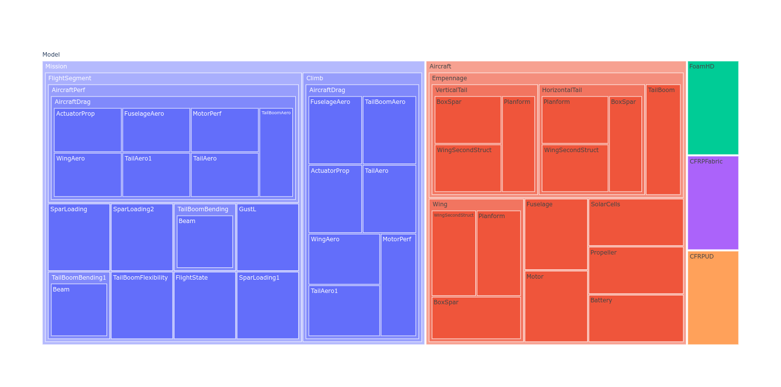
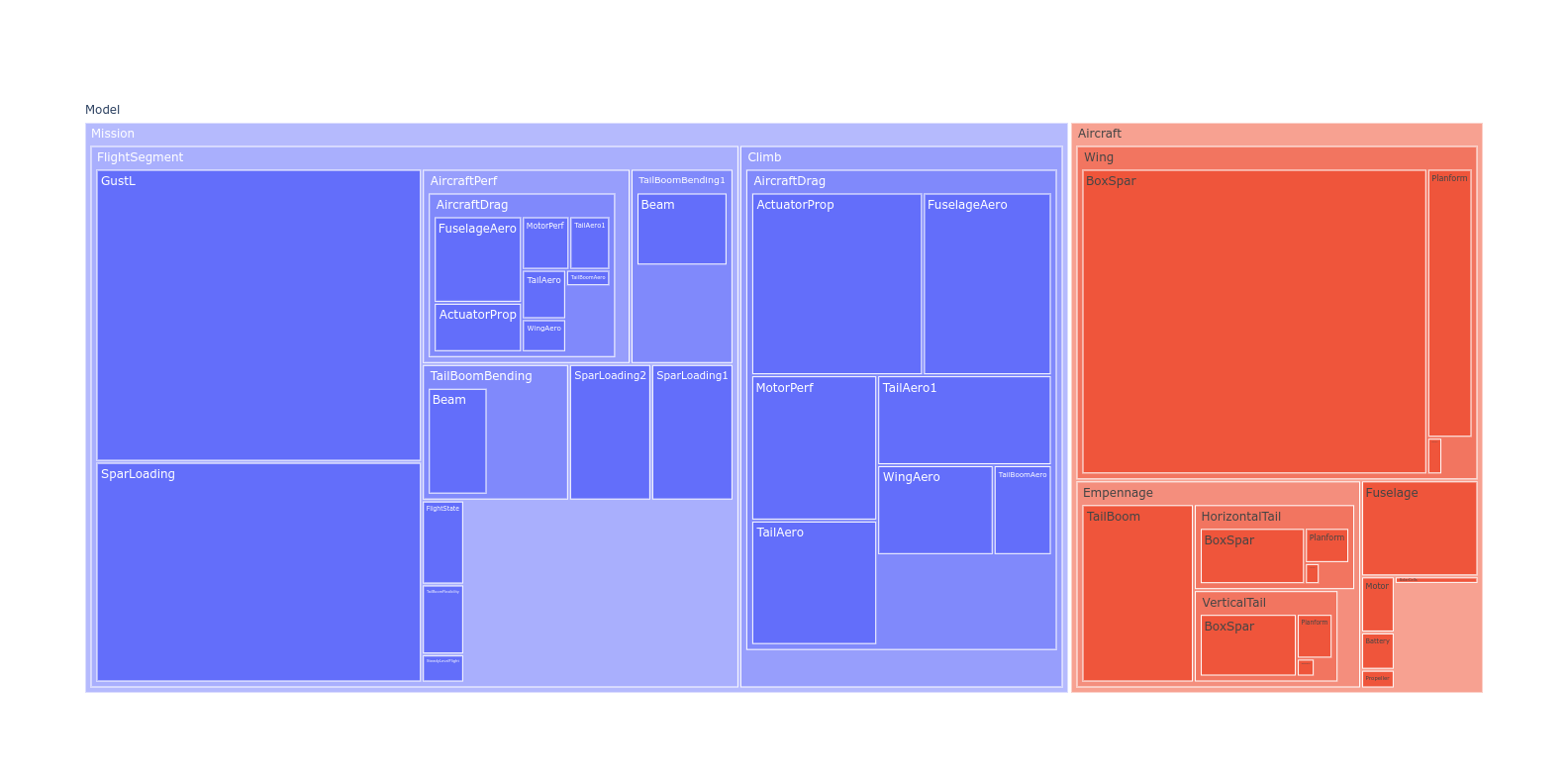
and, using sizing and counting by constraints instead of variables (the default):
fig = treemap(M, itemize="constraints", sizebycount=True)
plotly.offline.plot(fig, filename="sizedtreemap.html")
Variable Reference Plots
from solar.solar import *
Vehicle = Aircraft(Npod=3, sp=True)
M = Mission(Vehicle, latitude=[20])
M.cost = M[M.aircraft.Wtotal]
sol = M.localsolve()

from gpkit.interactive.references import referencesplot
referencesplot(M, openimmediately=True)
Running the code above will produce two files in your working directory:
referencesplot.html and referencesplot.json, and (unless you specify
openimmediately=False) open the former in your web browser,
showing you something like this:
Click to see the interactive version of this plot.
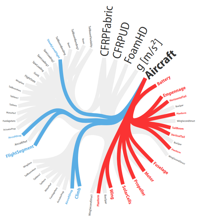
When a model’s name is hovered over its connections are highlighted, showing in red the other models it imports variables from to use in its constraints and in blue the models that import variables from it.
By default connections are shown with equal width (“Unweighted”). When “Global Sensitivities” is selected, connection width is proportional to the sensitivity of all variables in that connection to the importing model, corresponding exactly to how much the model’s cost would decrease if those variables were relaxed in only that importing model. This can give a sense of which connections are vital to the overall model. When “Normalized Sensitivities” is selected, that global weight is divided by the weight of all variables in the importing model, giving a sense of which connections are vital to each subsystem.
Sensitivity Diagrams
Requirements
- Jupyter Notebook
- ipysankeywidget
- Note that you’ll need to activate these widgets on Jupyter by runnning
jupyter nbextension enable --py --sys-prefix widgetsnbextensionjupyter nbextension enable --py --sys-prefix ipysankeywidget
- Note that you’ll need to activate these widgets on Jupyter by runnning
Example
from solar.solar import *
Vehicle = Aircraft(Npod=3, sp=True)
M = Mission(Vehicle, latitude=[20])
M.cost = M[M.aircraft.Wtotal]
sol = M.localsolve()

from gpkit.interactive.sankey import Sankey
Once the code above has been run in a Jupyter notebook, the code below will create interactive hierarchies of your model’s sensitivities, like so:
Explanation
Sankey
diagrams can be used to
visualize sensitivity structure in a model. A blue flow from a constraint to its parent
indicates that the sensitivity of the chosen variable (or of making the
constraint easier, if no variable is given) is negative; that
is, the objective of the overall model would improve if that variable’s
value were increased in that constraint alone. Red indicates a
positive sensitivity: the objective and the the constraint ‘want’ that
variable’s value decreased. Gray flows indicate a sensitivity whose
absolute value is below 1e-2, i.e. a constraint that is inactive for
that variable. Where equal red and blue flows meet, they cancel each
other out to gray.
Usage
Variables
In a Sankey diagram of a variable, the variable is on the right with its final sensitivity; to the left of it are all constraints that variable is in.
Free
Free variables have an overall sensitivity of 0, so this visualization shows how the various pressures on that variable in all its constraints cancel each other out; this can get quite complex, as in this diagram of the pressures on wingspan (right-click and open in a new tab to see it more clearly):
Sankey(sol, M, "SolarMission").diagram(M.aircraft.wing.planform.b, showconstraints=False)
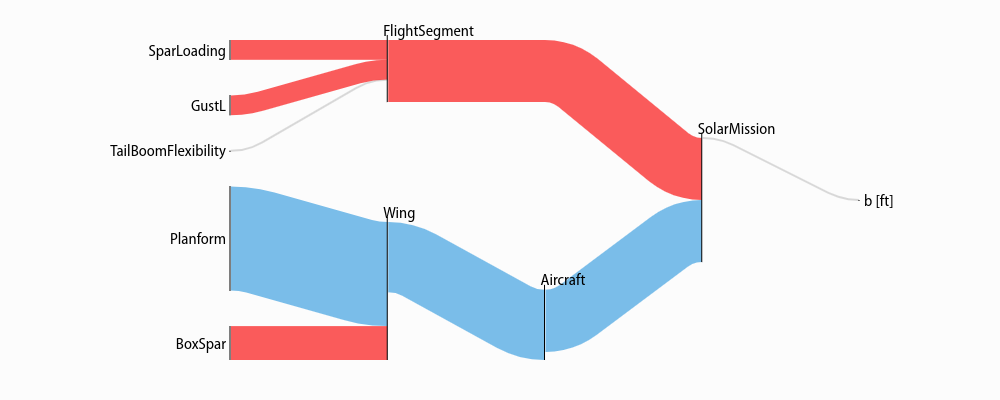
Gray lines in this diagram indicate constraints or constraint sets that the variable is in
but which have no net sensitivity to it. Note that the showconstraints
argument can be used to hide constraints if you
wish to see more of the model hierarchy with the same number of links.
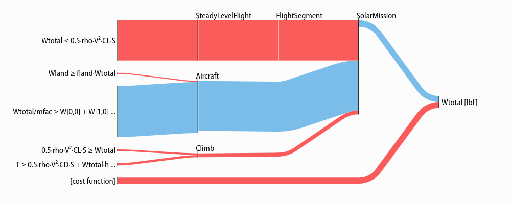
Variable in the cost function, have a “[cost function]” node on the diagram like so:
Sankey(sol, M, "SolarMission").diagram(M.aircraft.Wtotal)
Fixed
Fixed variables can have a nonzero overall sensitivity. Sankey diagrams can how that sensitivity comes together:
Sankey(sol, M, "SolarMission").diagram(M.variables_byname("tmin")[0], left=100)
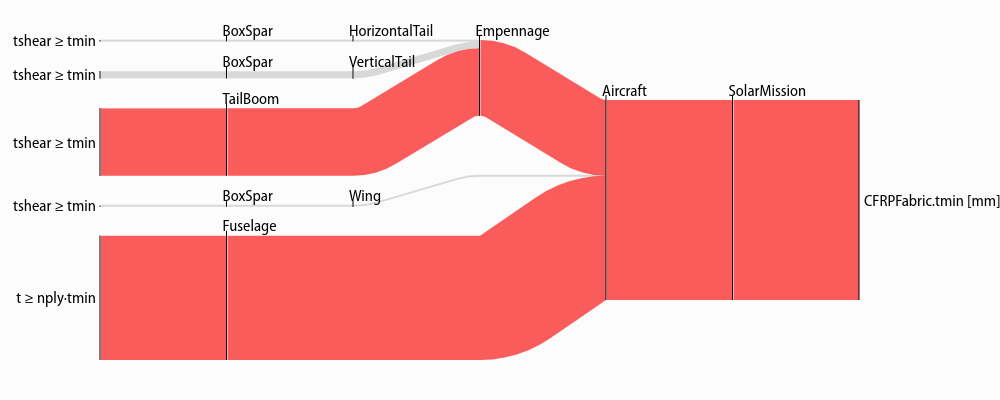
Note that the left= syntax is used to reduce the left margin in this plot.
Similar arguments exist for the right, top, and bottom margins:
all arguments are in pixels.
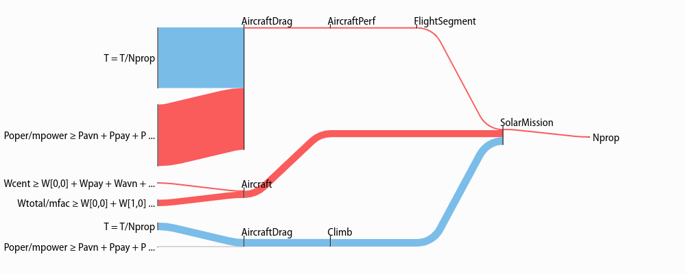
The only difference between free and fixed variables from this perspective
is their final sensitivity; for example Nprop, the number of propellers on the
plane, has almost zero sensitivity, much like the wingspan b, above.
Sankey(sol, M, "SolarMission").diagram(M["Nprop"])
Models
When created without a variable, the diagram shows the sensitivity of every named model to becoming locally easier. Because derivatives are additive, these sensitivities are too: a model’s sensitivity is equal to the sum of its constraints’ sensitivities and the magnitude of its fixed-variable sensitivities. Gray lines in this diagram indicate models without any tight constraints or sensitive fixed variables.
Sankey(sol, M, "SolarMission").diagram(maxlinks=30, showconstraints=False, height=700)
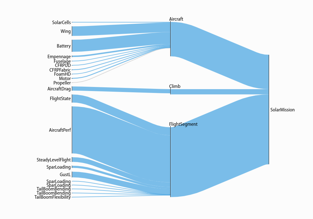
Note that in addition to the showconstraints syntax introduced above,
this uses two additional arguments you may find useful when visualizing large models:
height sets the height of the diagram in pixels (similarly for width),
while maxlinks increases the maximum number of links (default 20), making
a more detailed plot. Plot construction time goes approximately as the square
of the number of links, so be careful when increasing maxlinks!
With some different arguments, the model looks like this:
Sankey(sol, M).diagram(minsenss=1, maxlinks=30, left=130, showconstraints=False)
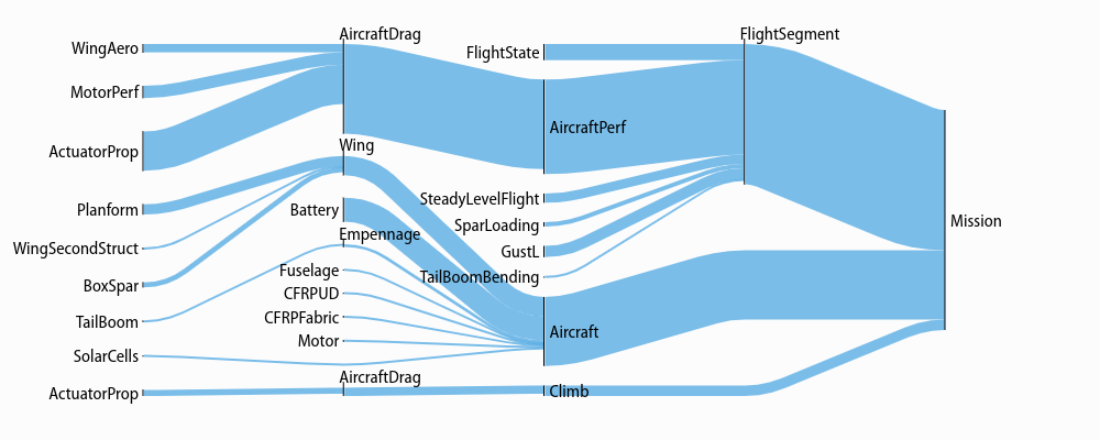
The only piece of unexplained syntax in this is minsenss. Perhaps
unsurprisingly, this just limits the links shown to only those whose sensitivity
exceeds that minimum; it’s quite useful for exploring a large model.
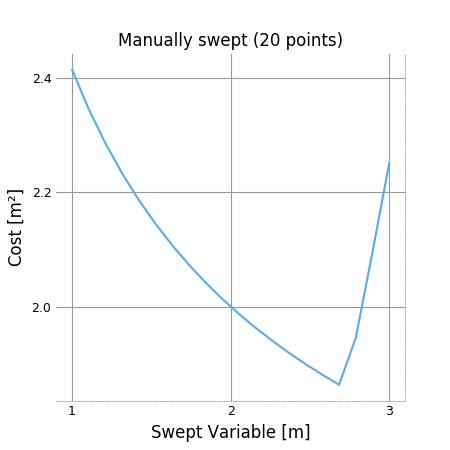
Plotting a 1D Sweep
Methods exist to facilitate creating, solving, and plotting the results of a single-variable sweep (see Sweeps for details). Example usage is as follows:
"Demonstrates manual and auto sweeping and plotting"
import matplotlib as mpl
mpl.use('Agg')
# comment out the lines above to show figures in a window
import numpy as np
from gpkit import Model, Variable, units
from gpkit.constraints.tight import Tight
x = Variable("x", "m", "Swept Variable")
y = Variable("y", "m^2", "Cost")
m = Model(y, [
y >= (x/2)**-0.5 * units.m**2.5 + 1*units.m**2,
Tight([y >= (x/2)**2])
])
# arguments are: model, swept: values, posnomial for y-axis
sol = m.sweep({x: np.linspace(1, 3, 20)}, verbosity=0)
f, ax = sol.plot(y)
ax.set_title("Manually swept (20 points)")
f.show()
f.savefig("plot_sweep1d.png")
sol.save()
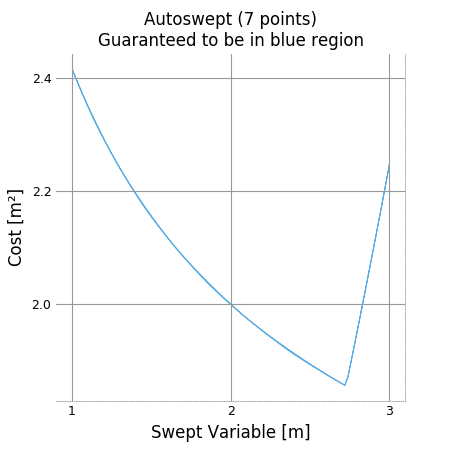
# arguments are: model, swept: (min, max, optional logtol), posnomial for y-axis
sol = m.autosweep({x: (1, 3)}, tol=0.001, verbosity=0)
f, ax = sol.plot(y)
ax.set_title("Autoswept (7 points)\nGuaranteed to be in blue region")
f.show()
f.savefig("plot_autosweep1d.png")
Which results in: